Author: Laurens

Please see also the project page for this paper.

Why cloud cover matters so much for EO data

Most of the Earth observation (EO) satellites currently in orbit are a little bit like fancy cameras: they measure a light spectrum. Unlike a regular camera, which just measures light intensity at the visible wavelengths humans can see (red, green and blue), the spectrometers (fancy cameras) on satellites measure light intensity at many different wavelengths, including ultraviolet and infrared. However, for most sensors, the light the satellite is trying to measure cannot pass through clouds, the same way you and I cannot see what is going on in the sky behind the clouds when we look up on a cloudy day. The clouds are basically photobombing our satellite imagery, which is not what we spent all that taxpayer money on! We want to know what is going on underneath the clouds!

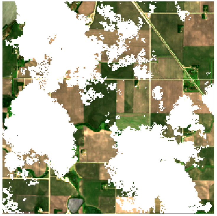
So when there are clouds in the sky, we can’t look through them, and that’s bad. Still, is it really that big a deal? Surely there are enough clear days to take a picture instead? Well, not really. First of all, at any given time, between 55% and 72% of the Earth is covered by clouds on average. You have to get quite lucky so that your one picture every 5 days (in the case of the popular Sentinel-2 satellite) exactly hits a gap in the cloud cover that covers the full spatial extent of your image. However, even this figure understates how big a problem cloud cover can be.

Clouds are not evenly spread over the Earth and its seasons. Countries near the equator are cloudy year-round, while countries further removed from the equator experience seasons. There, most of the cloud-free images we can capture are concentrated in the sunny summer, while in winter, it can be hard to get any feasible measurement at all for months on end.

For these reasons, we need methods capable of removing clouds from our satellite imagery, returning a full image with estimated values for the cloudy pixels.

VPint2 for cloud removal

We realised that our spatial interpolation method, VPint (see also its project page and plain-language explanation; in the following I will assume a knowledge of the original method), could be very well suited to this problem, offering substantial advantages over existing methods. However, this required us to add substantial extensions to the algorithm, prompting a name change to “VPint2”.

From predicted weights to exact reference weights

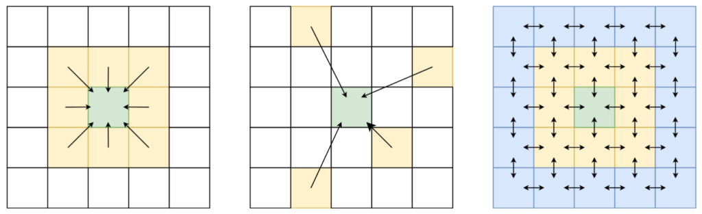
As you may recall, in WP-MRP, we predicted neighbour-specific weights based on some spatial features, to enable our spatial interpolation method to account for certain trends in the spatial structure. In EO settings, we can take this philosophy one step further: we don’t just need to model trends, we need to reconstruct an image with exact, sharp borders between objects.

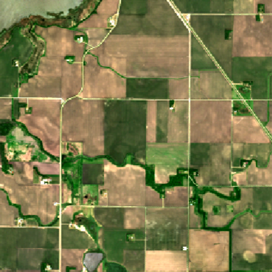
Thankfully, EO satellites keep taking pictures of the same area over and over again. While the situation on the ground may change over time (for example, trees turn from green, to golden brown, to completely without leaves), the spatial structure, and the “objects” it describes, remains relatively stable (a forest doesn’t disappear just because the state of the trees changes).

This is a property we can exploit to apply VPint2 to image reconstruction tasks instead of the general spatial interpolation tasks of the original VPint: we have the ultimate, extremely correlated weight features, available for direct computation in previous measurements! We simply compute the weights between all neighbours in a cloud-free reference image, and use those as the weights to perform VPint interpolation. This approach proved to be highly effective! However, there were still a few stability issues to iron out.

Improving stability and performance

There were two main issues that kept bugging us while working on this project.

First, we found that sometimes, strange colours from one object could “bleed” into another object. Although we assume that the spatial structure remains mostly stable over time, sometimes different objects can evolve differently over time. For example, imagine there were two objects in a summer reference image: a green forest, and a black asphalt road next to it. Next, in our cloudy autumn image, the forest turned golden brown, but the road remained black. The spatial structure remained mostly intact, because neighbours within objects were still very similar to one another, but at the borders, the spatial structure had changed: the relationship between objects had changed.

For this reason, we added a functionality we named identity priority. Basically, if we can choose between using information from the same object, or from a different object, we put a lot more faith into the information from pixels in the same object. We found that, in most cases, enabling this feature improved reconstruction performance — even in images where we couldn’t even see any visually apparent artefacts!

Second, sometimes the reconstruction would, for lack of a better word… go completely insane. Seriously, we would just get reconstructions with values in the order of magnitude 10^250. In the end, we figured out what had happened. Satellite data is flawed. Sometimes, there’s a pixel value that’s not quite right, either way too low, or way too high. To compute weights in the reference image, we divide one pixel value by another. If one of these values gets close to 0, we end up with some rather extreme multipliers, either very close to 0, or very large (depending on the direction). So, how did we solve this?

One step to reducing the impact of this issue is to simply constrain values not to exceed some maximal value, following similar preprocessing techniques to those used by other cloud removal methods. However, we also wanted a more elegant solution, so that a hard threshold is only used as a last resort. In the end, we created a feature we dubbed elastic band resistance.

Hopefully, the elastic band analogy makes the concepts easy to understand. Imagine the values of a pixel as the movement of an elastic band. Up to a certain point, you can move the band as far as you want. However, at some point, you hit the full length of the elastic band. If you want to move it further away, you can do so, but you will need to stretch the band to do it. At first, this is quite easy, but the further away you try to move, the more resistance the band will give to your push, and the more effort you will need for a relatively small movement.

This concept is what we applied to our method. Up to a certain threshold, pixel values could increase freely. After this threshold, any further increase in value is penalised based on how much the threshold is already exceeded, with larger excesses resulting in more resistance and smaller additional increases. We found this feature, combined with the “last resort” of clipped values, to effectively address the issues caused by faulty pixels and extreme weights.

Finally, in addition to identity priority and elastic band resistance, we greatly improved how fast VPint2 could perform cloud removal by adding parallel computing. Those who are curious about this aspect may be interested in the Bachelor thesis by my former student Dean, who worked on this topic.

Conclusion

In my experience, VPint2 is the easiest possible cloud removal method to use, short of just mosaicking past cloud-free pixel values (which, in terms of numerical performance, would be a very large sacrifice). I would encourage anyone who works with cloudy ground-level data to give it a try. After publication, I wrote a previous blog post as a quick tutorial for how to use the algorithm for your data. If you run into any issues despite these instructions, please feel free to get in touch, so that I can add or update material for further ease of use!

We are also currently looking into creating a cloudy time-series version of the method, removing the reliance on a single, fully cloud-free reference image. I’d also be interested in exploring avenues for getting the algorithm added to ESA’s SNAP tool, or data access point like Google Earth Engine or SentinelHub.

Please see also the project page for this paper.

What is spatial interpolation?

Suppose we want to know the concentration of fine dust concentrations throughout South Korea (and, trust me, we do). To this end, the Korean government has installed many fine dust measuring stations, whose data are then passed on to citizens through normal map- and navigation apps (like Naver maps) or dedicated fine dust mapping apps. The problem is that these concentrations will be different depending where you are in the country, making it a spatial problem, but the government cannot possibly install these sensors at every 10 square metres around the country: this would be expensive, get in the way of normal life, and difficult to install in, for example, inhospitable mountainous terrain.

As an alternative to putting sensors everywhere, it makes more sense to put them at a few important locations. For a random person walking around in Seoul, it does not matter if there is no measuring station exactly where they are currently standing. Instead, they can open a map, look at the closest measuring station, and assume that the air quality where they are standing is probably similar to that location.

In technical terms, this is called a ‘nearest neighbour interpolation’: you copy the value of the measurement that is closest to you. You could also look at the closest station in the other direction, and take the average value, or maybe give slightly more weight to the station that is closest; this would be a ‘linear interpolation’. If we perform this type of procedure for every possible point on the South Korean map, we have an ‘interpolated grid’: a full map of the country with estimated fine dust concentrations everywhere.

How VPint works

Suppose we are trying to estimate the fine dust concentration at a location Y1, right next to a location with a measuring station, which we call Y0. It makes sense to say that the concentration at our location, Y1, would probably be quite similar to that of the measuring station Y0, right? There may be some minor changes, but usually, the value will be close. Now we want to know the value of the location Y2, which is next to the location Y1 that we were interested in before. Here we can repeat the same thought process: the concentration at Y2 will probably be quite similar to that of Y1, but possibly with some minor differences.

In fact, we can keep this going indefinitely. Starting from a source location, like the measuring station at Y0, we can keep passing on this value to neighbouring locations right next to the previous location. Every time we pass on this message, we are a little less sure about the value that comes out. This is represented using a weight: every time we pass on the message, we “discount” the value passed on to the next neighbour. At the first step, this may not be a big deal; however, as we pass the message through more and more locations, these discounts really start adding up. While doing so, we naturally stop paying too much attention to the value passed from Y0, and instead give more priority to other values. If there is a value coming in from a different, closer location, we may put more faith in the messages passed from there; if there are no more messages from measured values, we just slowly move towards just predicting the average (mean) value.

Because we are working with spatial data, every location has a neighbour above, below, to the left and to the right. To pass a message, we update the value of a location to be the average of the signals (discounted values) it receives, which effectively merges the information received from every direction. However, this only works for direct neighbours; if we really want to spread (propagate) these messages further, we have to keep repeating this update procedure. What started as a simple update rule now results in a large system of invisible flows of information between all locations!

SD-MRP and WP-MRP

The procedure I described above is what we do in the “SD-MRP” version of the VPint algorithm. The SD refers to a “static discount”, which we use to represent a decreasing confidence in our estimations the more often we pass a message between two neighbours, while “MRP” refers to Markov reward processes. This mathematical concept, which we took inspiration from to base our method on, has the nice property that if we keep repeating the update rule described above, we eventually reach a stable configuration where new updates don’t really change anymore.

In WP-MRP, where WP refers to “weight prediction”, we can do a neat trick to get even more accurate results. Suppose now that we are still in the same problem setting (fine dust concentrations, scattered measuring stations), but now we have access to some extra data, such as the number of motor vehicles at every location. If this extra data (motor vehicles) is correlated with the target variable (fine dust concentration), we can customise the flow of information from one neighbour to the next.

For example, suppose that one location is situated in a busy urban area, but with a mountain park right next to it. Using SD-MRP, we would pass the fine dust concentration from the urban area to the mountain park, and just discount it to signify that we are less confident in that information. However, if we know that the urban area contains many motor vehicles, while the mountain contains almost none, we can change the weight to signify that we expect fine dust levels to be much lower in a mountain area than in its urban counterpart (which we approximate using motor vehicles). Instead of slowly trending towards the average values, we can instead say that the value should be much lower than that of the urban area, perhaps even lower than the mean.

We can use machine learning to learn the relationship between the features describing two neighbouring locations (like the number of cars in both), and the spatial weight between those locations (which we can see in cases where we do know the values of both). This machine learning model can then predict the spatial weight between two locations, if you only pass the right input data that it expects.

Conclusion

This is, in a nutshell, how our method works! I hope this explanation was helpful; if you have any further questions, please feel free to reach out via the comments, or via email.