Please see also the project page for this paper.
What is spatial interpolation?
Suppose we want to know the concentration of fine dust concentrations throughout South Korea (and, trust me, we do). To this end, the Korean government has installed many fine dust measuring stations, whose data are then passed on to citizens through normal map- and navigation apps (like Naver maps) or dedicated fine dust mapping apps. The problem is that these concentrations will be different depending where you are in the country, making it a spatial problem, but the government cannot possibly install these sensors at every 10 square metres around the country: this would be expensive, get in the way of normal life, and difficult to install in, for example, inhospitable mountainous terrain.
As an alternative to putting sensors everywhere, it makes more sense to put them at a few important locations. For a random person walking around in Seoul, it does not matter if there is no measuring station exactly where they are currently standing. Instead, they can open a map, look at the closest measuring station, and assume that the air quality where they are standing is probably similar to that location.
In technical terms, this is called a ‘nearest neighbour interpolation’: you copy the value of the measurement that is closest to you. You could also look at the closest station in the other direction, and take the average value, or maybe give slightly more weight to the station that is closest; this would be a ‘linear interpolation’. If we perform this type of procedure for every possible point on the South Korean map, we have an ‘interpolated grid’: a full map of the country with estimated fine dust concentrations everywhere.
How VPint works
Suppose we are trying to estimate the fine dust concentration at a location Y1, right next to a location with a measuring station, which we call Y0. It makes sense to say that the concentration at our location, Y1, would probably be quite similar to that of the measuring station Y0, right? There may be some minor changes, but usually, the value will be close. Now we want to know the value of the location Y2, which is next to the location Y1 that we were interested in before. Here we can repeat the same thought process: the concentration at Y2 will probably be quite similar to that of Y1, but possibly with some minor differences.
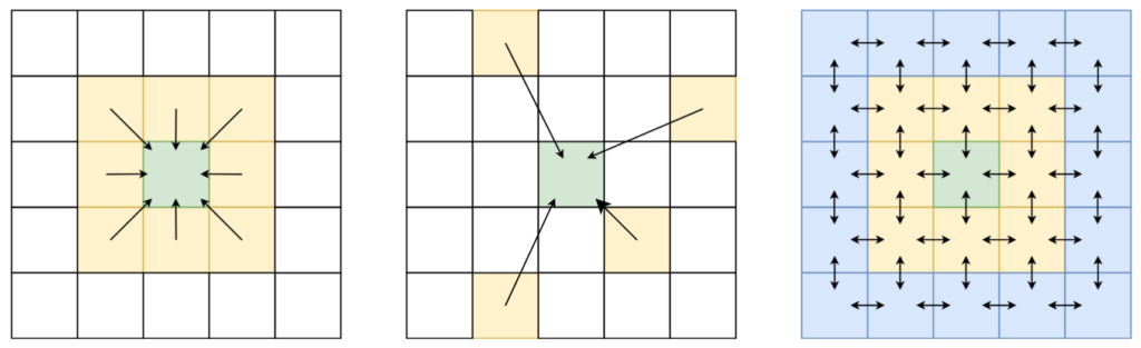
In fact, we can keep this going indefinitely. Starting from a source location, like the measuring station at Y0, we can keep passing on this value to neighbouring locations right next to the previous location. Every time we pass on this message, we are a little less sure about the value that comes out. This is represented using a weight: every time we pass on the message, we “discount” the value passed on to the next neighbour. At the first step, this may not be a big deal; however, as we pass the message through more and more locations, these discounts really start adding up. While doing so, we naturally stop paying too much attention to the value passed from Y0, and instead give more priority to other values. If there is a value coming in from a different, closer location, we may put more faith in the messages passed from there; if there are no more messages from measured values, we just slowly move towards just predicting the average (mean) value.
Because we are working with spatial data, every location has a neighbour above, below, to the left and to the right. To pass a message, we update the value of a location to be the average of the signals (discounted values) it receives, which effectively merges the information received from every direction. However, this only works for direct neighbours; if we really want to spread (propagate) these messages further, we have to keep repeating this update procedure. What started as a simple update rule now results in a large system of invisible flows of information between all locations!
SD-MRP and WP-MRP
The procedure I described above is what we do in the “SD-MRP” version of the VPint algorithm. The SD refers to a “static discount”, which we use to represent a decreasing confidence in our estimations the more often we pass a message between two neighbours, while “MRP” refers to Markov reward processes. This mathematical concept, which we took inspiration from to base our method on, has the nice property that if we keep repeating the update rule described above, we eventually reach a stable configuration where new updates don’t really change anymore.
In WP-MRP, where WP refers to “weight prediction”, we can do a neat trick to get even more accurate results. Suppose now that we are still in the same problem setting (fine dust concentrations, scattered measuring stations), but now we have access to some extra data, such as the number of motor vehicles at every location. If this extra data (motor vehicles) is correlated with the target variable (fine dust concentration), we can customise the flow of information from one neighbour to the next.
For example, suppose that one location is situated in a busy urban area, but with a mountain park right next to it. Using SD-MRP, we would pass the fine dust concentration from the urban area to the mountain park, and just discount it to signify that we are less confident in that information. However, if we know that the urban area contains many motor vehicles, while the mountain contains almost none, we can change the weight to signify that we expect fine dust levels to be much lower in a mountain area than in its urban counterpart (which we approximate using motor vehicles). Instead of slowly trending towards the average values, we can instead say that the value should be much lower than that of the urban area, perhaps even lower than the mean.
We can use machine learning to learn the relationship between the features describing two neighbouring locations (like the number of cars in both), and the spatial weight between those locations (which we can see in cases where we do know the values of both). This machine learning model can then predict the spatial weight between two locations, if you only pass the right input data that it expects.
Conclusion
This is, in a nutshell, how our method works! I hope this explanation was helpful; if you have any further questions, please feel free to reach out via the comments, or via email.
Leave a Reply